バイオリンプロットをプログラムで描いてみる

こんにちは。この記事がちょうど月末の投稿になるので、「グラフを描いてみる」シリーズをあと1回続けることにします。
今回はバイオリンプロットです。少し前に箱ひげ図を描いてみました。

箱ひげ図は、最大値・最小値・四分位数がわかるような、とても工夫されたグラフだと思います。
しかし、データの分布が見えにくくなってしまっているように思います。
そこで、バイオリンプロットというグラフを描いてみることにします。
どのようなグラフかは、見た方が早いので実際に描いてみます。
目次
Python + seaborn + matplotlib で描くバイオリンプロット
はじめに、seabornを使って描いていきます。
import seaborn
import matplotlib.pyplot
iris = seaborn.load_dataset( 'iris' )
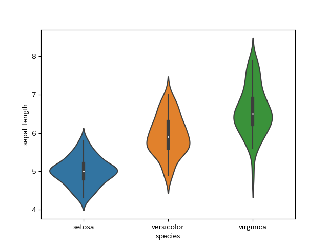
seaborn.violinplot( x=iris['species'], y=iris['sepal_length'] )
matplotlib.pyplot.show()
このプログラムで、次のようなグラフが描けます。
Python + seaborn + matplotlib でバイオリンプロットを工夫してみる
上のバイオリンプロットでは、四分位数がわからなくなっているので、表示してみます。
そのプログラムです。violinplotのパラメータに inner="quartile" を付けました。
import seaborn
import matplotlib.pyplot
iris = seaborn.load_dataset( 'iris' )
seaborn.violinplot( x=iris['species'], y=iris['sepal_length'], inner="quartile" )
matplotlib.pyplot.show()
次のようなグラフになります。

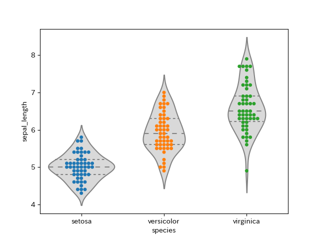
さらに、元のデータの分布をドットで表示するスウォームプロットを追加してみます。
(バイオリンプロットの色はグレーにしました。)
import seaborn
import matplotlib.pyplot
iris = seaborn.load_dataset( 'iris' )
seaborn.violinplot( x=iris['species'], y=iris['sepal_length'], inner="quartile", color="0.85"  )
seaborn.swarmplot( x=iris['species'], y=iris['sepal_length'] )
matplotlib.pyplot.show()
出来上がったグラフです。
R で描くバイオリンプロット
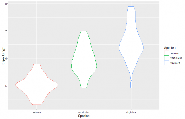
次にRで描いてみます。ggplot2 を使います。
library( ggplot2 )
data( iris )
v <- ggplot( iris, aes( x= Species, y=Sepal.Length, color=Species )) +
    geom_violin()
plot(v)
次のようなグラフが描けます。
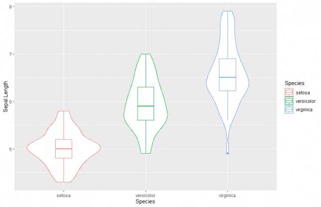
箱ひげ図を重ねてみます。
library( ggplot2 )
data( iris )
v <- ggplot( iris, aes( x=Species, y=Sepal.Length, color=Species )) +
    geom_violin() +
    geom_boxplot( width=0.2 )
plot(v)
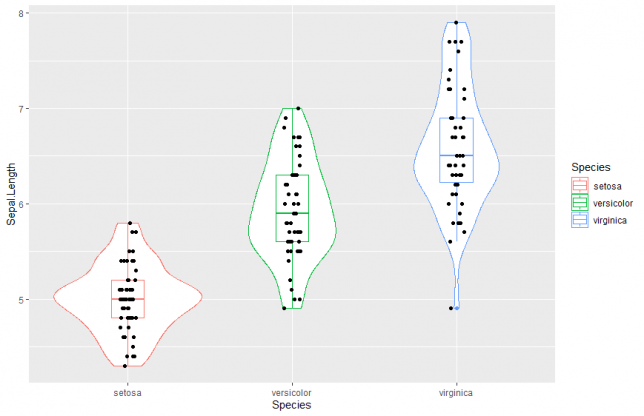
さらにビースウォームを重ねてみます。
library( ggplot2 )
data( iris )
v <- ggplot( iris, aes( x= Species, y=Sepal.Length, color=Species, trim=FALSE )) +
    geom_violin() +
    geom_boxplot(width=0.2) +
    geom_point( position=position_jitter( width=0.05, height=0 ), color="black", stackdir="center" )
plot(v)
今回はこれでおしまいにします。それでは、また。